FairChoices Methods
Table of Contents
- Summary
- Health impact model
- Mathematical details of health impact model
- Health effect models
- Demographic projection model
- Cost model
- Limitations
Summary
FairChoices is a deterministic mathematical model of the population that includes demographic and epidemiological parameters taken from international data sources. The model calculates the potential impact of interventions by changing rates of disability and mortality from various causes as a function of the effectiveness of the interventions (taken from the literature) and changes in population coverage (e.g., scaling up intervention X from 30% coverage in 2025 to 80% coverage in 2050).
Intervention costs are taken from the literature and adjusted to different country settings. The demographic and epidemiological data identify the population in need of each intervention, which along with the coverage assumptions informs the estimates of aggregate costs.
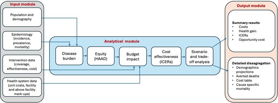
Fig 1. Analytical process of FairChoices system
Health impact model
Overall structure of health impact model
Steps that are used in calculation of lifetime health effects:
- Defining age cohorts
1-year age- and sex-specific mortality and disability rates are adjusted according to increase in target coverage.
Future birth cohorts are projected based on baseline mortality and fertility. - Health-adjusted life expectancy (HALE) calculations
For each age cohort, current and future, we calculate sex-specific HALE in the baseline scenario (i.e. no change in coverage) and in the adjusted scenario (i.e. with interventions scaled to target coverage). - Cohort-level HYs gained
Sex-specific HYs gained are calculated for each cohort in the population by:
HYcohort,sex = Ncohort,sex(HALEcohort,sex(target) – HALEcohort,sex(baseline)), where HALEcohort,sex is calculated for an average individual of a specific cohort and sex.
- Total HYs gained
Total HYs gained are obtained by summing all the sex- and cohort-specific HYs:
HYtotal = cohort, sex(HYcohort,sex)
Steps that are used in calculation of deaths averted (statistical lives saved):
- Defining age cohorts
1-year age- and sex-specific mortality and disability rates are adjusted according to increase in target coverage.
Future birth cohorts are projected based on baseline mortality and fertility. - Mean change in mortality rates (Mx)
Calculate mean statistical lives saved (SLS) in each current and future age cohort by:
Mx = Mx(baseline) – Mx(target) - SLS per age cohort
Calculate cohort-specific SLS by summing gains for each current and future age cohort:
SLScohort=popcohort(baseline)Mxcohort
- Total SLS
Total SLS are obtained by summing summing sex- and cohort-specific SLS:
SLStotal = cohort, sex(SLScohort,sex)
- One artifact with this methodology is that the population is dynamic, meaning births are entering future age cohorts, and interventions improving SLS may create larger future older age cohorts, and this is why you may see negative SLS in older cohorts for some interventions.
More details about the specific methods are below:
Mathematical details of health impact model
The FairChoices model uses a lifetime perspective on health. This is to capture benefits that last well beyond the implementation period from interventions like HPV vaccination of adolescents, kidney transplant, and obstetric fistula surgery. We do this using a model based on standard lifetable methodology, where input on demography and epidemiology is based on the World Population Prospects and the Global Burden of Diseases and Injuries study (GBD), input on the coverage and effects of the interventions is compiled from the medical literature and other data sources (e.g., WHO Global Health Observatory, World Bank Open Data).
Conceptually, we first assume that without implementing interventions, cause-, sex-, and age-specific mortality and morbidity will remain unchanged into the future. Then we calculate healthy life-expectancy (HLE) for each cohort (i.e., the people born the same year) alive today and for the cohorts that will be born during the scale-up period.
Assuming a scale-up period of 25 years and that mortality is 100% at age 100, we then need to consider 126 cohorts ( C0 through C100 are the cohorts that are alive today, and C-1 through C-25 the cohorts that will be born the next 25 years). We can now present the mortality of these cohorts as follows:

Mx denotes the mortality from age x to age x+1. As seen, M100=1 for all cohorts.
Cy denotes the cohort. A negative y is used if the cohort has not yet been born. For example, C-25 denotes the cohort that will be born in 25 years.
One table is constructed for each sex.
Corresponding tables are also constructed for disability (i.e., morbidity), based on the age- and sex-specific disability weights provided by GBD:

Dx denotes the disability from age x to age x+1. Note that D100 is not 1.
Cy denotes the cohort. A negative y is used if the cohort has not yet been born. For example,C-25 denotes the cohort that will be born in 25 years.
Once these matrices have been populated, we introduce interventions that are specified to act on a condition (defined as one of the GBD causes of death or disability) within a sex- and age-specific population and have a duration where they are effective. For treatment of acute conditions, the duration is one year, whereas for interventions like vaccines and obstetric fistula surgery the duration is longer and may even be lifelong.
Each intervention reduces mortality, disability, incidence, or prevalence of one or more conditions. The crude effect of the intervention,ecrude, is adjusted to account for the change in coverage during the scale-up period and the fact that the observed mortality or disability is being experienced mostly among those who are not currently covered by the intervention (though this also depends on how effective the intervention is among those who are covered).
We thus use the formula:
eadj = ecrude (covtarget – covbaseline)1 – (ecrude covbaseline)
Where: ecrude and eadj are expressed as relative risk reductions and covbaseline and covtarget are coverage at baseline and target.10
Further, Mx can be divided into the cause-specific mortality from the targeted condition and what we call “background mortality”, which is the risk of dying from any other cause:
Mx = Mx,background- Mx,cause
Applying the intervention, we get:
Mx,adjusted = Mx,background+ Mx,cause (1- eadj)
As seen, if e_adj=1, cause-specific mortality is reduced to zero in the targeted population. If a total of K interventions target the same condition, we get
Mx,adjusted=Mx,background+Mx,cause (1-eadj,1)(1- eadj,K)
where eadj,) is the effect of the kth. This ensures that cause-specific mortality cannot be less than 0. We make similar calculations for interventions that reduce disability. We also scale up coverage of the intervention gradually over time. This means that the full effect will not be felt until the last year, so that the age-specific mortalities (and disabilities) in different cohorts (C-25 through C100 ) will be affected differently. Hence, to make intervention-“adjusted” versions of the matrices above, each cell is now both age- and cohort-specific.
For mortality:

M(x,y) denotes the mortality from age x to age x+1 in cohort y. As seen, M100=1 for all cohorts.
Cy denotes the cohort. A negative y is used if the cohort has not yet been born. C-25 denotes the cohort that will be born in 25 years.
For disability:

Dx,y denotes the disability from age x to age x+1 in cohort y. Note that D100 is not 1.
Cy denotes the cohort. A negative y is used if the cohort has not yet been born. For example,C-25) denotes the cohort that will be born in 25 years.
The statistical lives saved (SLS) for the individuals in cohort y is given as:
SLSy=Ny x y=0100(Mx-Mx,y)
where Mx and M(x,y) are from the baseline and adjusted matrices, multiplied by respective population counts. If we want to limit ourselves to counting SLS, for example, during the scale-up period, this is done by changing the start and end values of the index x.
Summing over y gives the total SLS
Total SLS=∑_(y=-25)^100〖SLS_y 〗
Calculating lives saved under a certain age, X, we can first calculate the risk of dying before X for each cohort. At baseline, this risk is
P_y (X|baseline)=1-(1-M_max(y,0) )×⋯×(1-M_X )
Where max(y,0) ensures that we do not consider pre-birth mortalities for cohorts C_(-25) through C_(-1) or the mortality of years past for cohorts C_1 through C_100. After scaling up the interventions, the risk becomes
P_y (X|adjusted)=1-(1-M_max〖(y,0),y〗 )×⋯×(1-M_(X,y) )
Now, lives saved below X is the sum
Under-X lives saved =∑_(y=-25)^100 ((P_y (X|baseline)-P_y (X│adjusted))×N_y )
Finally, for an individual in cohort y, we can calculate healthy life expectancy (HLE) based on the mortality rates and disability weights in the baseline matrices (i.e., HLE_(baseline,y)) and in the adjusted matrices (i.e, HLE_(adjusted,y)). The healthy life-years (HLYs) gained is now simply
HLYs gained_y=HLE_(adjusted,y)-HLE_(baseline,y)
Total HLYs gained from scaling up one or more interventions then becomes the sum
Total HLYs gained=∑_(y=-25)^100 (HLYs gained_y×N_y )
where N_y is the number of individuals in cohort y.
PRM denotes how long an intervention is effective after it has been administered. E.g., an intervention will have an effect for scaleup-period + PRM years for the people affected by the intervention.
Health effect models
In FairChoices, we use 9 different effectiveness models:
- High urgency effects
Interventions used in critical care situations where timing is important, and may affect mortality and disability.
(e.g. treatment of pneumonia or diarrhea) - Future cohort prevention
Interventions given at one point of time, but effects come later in life of the cohort.
(e.g. vaccines) - Treatment AND prevention effects
Interventions given at one point of time, but effects both accrue to people with a disease and benefits later in life of the cohort.
(e.g. treatment of Hepatitis C (effect on HepC and future liver cancer, Apocillin to treat StrepB tonsillitis and prevent Rheumatic heart disease) - Non curative – short term effects
Chronic care interventions saving lives, may also improve disability, and increasing prevalence
(e.g. HIV treatment, antihypertensives) - Non curative – long term effects
Interventions saving lives, may also improve disability, and has effects beyond the interventions period (e.g. orthopedic surgery, kidney transplant, cancer) - Non curative – disability only
Chronic care interventions only affecting disability (e.g. treatment of rheumatoid arthritis) - Fertility effect
Interventions affecting fertility.
(e.g. family planning) - Indirect effect – quality
Interventions with indirect effectiveness on other interventions, necessary to achieve optimal quality of affected interventions
(e.g Essential Emergency Critical Care) - Indirect effect – access
Important interventions without direct health effects per se, necessary to detect conditions and to achieve target coverage.
(e.g. universal screening, diagnostics)
More details are explained below:
Prevent acute condition for full cohort over a period of more than 1 year (E.g., vaccines)
Action: Reduce mortality and disability for whole cohort for duration of PRM (PRM>1)
Example: If PRM=15 for BCG vaccine to infants, and the intervention is provided to infants in a birth cohort, then prevalence of TB will be reduced in this whole birth cohort for 15 years. After 15 years, we assume that mortality in the birth cohort reverts back to baseline mortality (i.e., mortality without any intervention). In other words, once the children in the vaccinated birth cohort reach the age of 16, we assume that they are not protected against TB. Further, we assume that the reduction in prevalence is the same every year during the 15 years (PRM).
Immediate treatment of incident cases of acute conditions or short-term treatment of non-deadly chronic conditions (E.g., treatment of diarrhea or arthritis)
Action: Reduce mortality and/or disability for all ages treated in the year of treatment (PRM=1, may be necessary to separate incidence from prevalence)
Short-term treatment of deadly chronic conditions (E.g., treatment of HIV, dialysis for CKD, diabetes treatment)
Action: Reduce mortality for all age-groups in the year of treatment (PRM=1). After scaleup-period is done, mortality must increase for a short period because of “owed mortality”.
Long-term treatment of deadly chronic conditions (E.g., kidney transplant, cancer treatment)
Action: Reduce mortality for all age-groups for duration of PRM (PRM>1). The effect within cohort is reduced by a certain fraction per year to account for the fact that new cases in years 2 to PRM were not treated the initial year.
Example: If we provide everyone aged 50 in the year 1 (e.g., 2024) in need of a kidney transplant with a new kidney, the mortality in that age cohort will be reduced for 15 years (assuming that PRM=15). However, because the treatment provided in year 1 does not affect mortality for new cases in year 1 in the same age cohort, the effect in year 2 is effect year 1 multiplied by 1/2. This is based on the assumption that incidence will be approximately the same every year. The effect in year T, will be (effect year 1)*(1/T). Hence, in year 15, the reduction in mortality of the cohort aged 50 in year 1 (who are 64 in year 15), will be (effect year 1)*(1/15). If coverage is kept at the same level each year, the effect on mortality will remain the same for the duration of the period with increased coverage.
Contraception and family planning
Action: Reduce fertility for relevant ages treated in the year of treatment based on met need.
Demographic projection model
The above approach describes how to compute changes in health outcomes in a static population, with one major output being changes in age-, sex-, and cause-specific mortality rates. To translate these into “real” projected populations, and to account for changing population size due to fertility, we employ a demographic model that uses the cohort component projection method (CCPM). The CCPM is based on the primary determinants of population dynamics: fertility, mortality, and migration. The initial population structure, segmented by sex and categorized by discrete age groups from 0 to 100 years, is based on the 2022 release of the World Population Prospects (WPP) by the United Nations Population Division.
We initiate our projections with a detailed population age structure, delineated by sex and organized into single-year age brackets, ranging from 0 to 100 years. For fertility, we utilize the age-specific fertility rates (ASFR) provided by the WPP. The number of births is calculated by multiplying the number of females in each reproductive age group (typically ages 15 to 49) by the corresponding ASFR, and integrating across all reproductive ages to include the entire fertility span:
B(t)=∫_(a=15)^49▒〖〖ASFR〗_f (a,t)×P_f (a,t)da〗
However, due to the granularity of the data and the necessity for computational efficiency, we opt for a discrete approximation:
B(t)=∑_(a=15)^49▒〖〖ASFR〗_f (a,t)×P_f (a,t)〗
For mortality changes, we use the life tables that are based on the population size and structure and mortality patterns in the starting year of the analysis. The survivorship of individuals in the population is calculated using life table survivor rates, S(a,t), which give the probability of surviving from age a to age a+1. This allows us to compute the population at each age and sex in the subsequent year:
P_s (a+1,t+1)=P_s (a,t)×S_s (a,t)
Here, 𝑠 denotes the sex subscript, distinguishing between male (𝑚) and female (𝑓) populations.
Finally, the population projection is refined by incorporating net migration, M_s (a,t), for each age and sex:
P_s^* (a+1,t+1)=P_s (a+1,t+1)+M_s (a,t+1)
The total adjusted population for each age and sex in the subsequent year is thus the sum of the survivors from the preceding year and the net migrants. These equations collectively form the foundation of our demographic projections, providing a comprehensive account of how a population would evolve differently in the baseline and adjusted scenarios, depending on the interventions and coverage targets chosen.
Cost model
Our cost model generally follows the approach outlined by Watkins and colleagues[1] in DCP3. In brief, we searched the literature for estimates of the annual unit cost (defined per population or per case treated, depending on the intervention) of each of the interventions in FairChoices. (Data sources for each intervention are also provided.) To each intervention-specific unit cost ci,lit presented in the literature, we added in health system strengthening costs to each unit cost estimate c and intervention i.
ci = (1 + α) · ci,lit · (1 + β)
As in DCP3, α is a markup reflecting facility-level “indirect” costs (e.g., utilities, maintenance, administration, laboratory and pathology services, etc.), calculated based on Access, Bottlenecks, Costs, and Equity (ABCE) Project data from the Institute for Health Metrics and Evaluation. The α markup was calculated by intervention platform (7.4% for outpatient facilities and 27% for inpatient facilities) based on estimates of the proportion of total cost from infrastructure, administration, and nonmedical services in Kenya, Uganda, and Zambia.
The β is a markup reflecting “above-facility” health system costs including supply chain, financing, governance and administration, and health information systems, set at 17% as per DCP3. We included these costs in our model to reflect the importance of investing in health systems to support delivery of specific interventions. (These costs were only added on when they were not included in the original studies.)
Unit costs were taken from representative studies based in single countries. These costs were extrapolated to all other LICs and LMICs under the assumption that traded goods would not vary across countries, on average, and non-traded goods and services would vary in proportion to health worker salaries. Hence the unit cost in the target country y with health worker salary Sy estimated as
ci,y = δ · ci,x · (Sy / Sx) + (1 − δ) · ci,x,
for unit cost ci in the originating country x with gross national income per capita Sx and a traded proportion of total unit cost equal to δ. On average, δ was around 0.3, but we computed this proportion separately for each unit cost data point used. In a few instances, we used updated drug prices from Management Sciences for Health (MSH) in lieu of drug costs cited in the study (see below), and so the study-specific δ was adjusted further as necessary.
All costs were converted and inflated to latest world bank year US dollars using procedures described by Watkins and colleagues[1]. Unit cost estimates were combined with estimates of populations in need and estimates of population coverage to estimate intervention costs at a population level, Ci,pop:
Ci,pop = Σk=1n ci,k · wi,k · pi,k
where wi,k is the proportion of the target population covered by cost line k of intervention i and pi,k is the estimated number of persons treated by cost line k of intervention i, also referred to as the “population in need.” The population in need of each intervention is usually derived from disease-specific incidence or prevalence estimates, with some adjustments based on the properties of the intervention. For example, if 80% of persons with disease X are eligible for intervention i, we multiply the prevalence of disease X by 0.80 (we call this the “treated proportion”).
We assumed that ci remained constant (in latest world bank data year US dollars) throughout the analytic horizon, but we used year-specific estimates of pi from the demographic model and year-specific values of wi specified in our projection model (see above). This approach allowed us to generate a stream of population-level costs for all interventions, summed together to calculate the overall “package” cost. The summation was done by year for the baseline scenario (i.e., no change in wi) and various intervention scenarios where wi was increased as a function of time. The difference between these two streams of costs, then, is the “incremental cost” of the intervention scenario, which corresponds to an improvement in health that results from an increase in intervention coverage over the same time.
We discount cost by 5% and health by 0% in cost effectiveness ratios. We don’t discount either in the finance tab. Discounting cost by 5% means everything is given in current USD, however next years cost is modified by 1/1.05, the cost in two years by 1/1.052, etc up until 1/1.055 in the fifth and last year.
References
Limitations
A significant limitation in our cost modeling approach is the lack of empirical data concerning economies (and diseconomies) of scope and scale in the context of Non-Communicable Disease (NCD) interventions. While health economists generally recognize the potential for economies of scope in interventions with similar delivery characteristics, empirical validation and quantification of such economies have proven challenging. Economies of scale are more readily demonstrated in national-level programs for communicable diseases, but very little is known about the cost of NCD programs nationally and how the unit costs change with variations in population coverage. Accordingly, our cost model assumed constant marginal costs concerning coverage, though marginal costs likely differ at very low and high coverage levels. Despite this limitation, our analysis focused on (10-20%) increases in coverage from 2023 to 2030, providing a more justifiable basis for assuming constant marginal costs.